Joint Research Group Macromolecular Crystallography
Usage
The program and its necessary packages is installed on one of our servers at HZB and is therefore accessible from every computer connected to our MX linux network. It can be opened with the command xfeplot.
To load a new scan click on File in the top left menu bar and then Open in the drop down menu.
Browse to your file and load it. Otherwise you can also enter the command xfeplot <yourfile> in a command line. XFEplot can read .dat and .mca files. The spectrum will be displayed in the central Widget, by drawing the counts over the specific energy. For manual analysis, the whole periodic table of elements (PSE) is depicted underneath the window in which the spectrum is displayed. For each of the elements the expected X-ray fluorescence peaks are hard-coded in a table. By just clicking on the respective element in the PSE, the expected peaks can be added to (and removed from) the spectrum.
Search
The search analysis is semi-automatic. A peak search routine is applied to the raw spectrum. All observed peaks are compared with expected Kα or Lα values, which are stored internally. In order to improve the prediction accuracy the respective Kß or Lβ peaks are compared as well. In addition to the simple search routine an automated fitting of the observed peaks using a Gaussian function has been implemented to get better peak values. This is carried out by utilizing the open source library SciPy.
Smoothing
XFEplot allows the user to perform a few more things with the raw data. A smoothing function has been implemented to average out background counts. Although the smoothed spectra look more appealing visually, smoothing does lead to a slight degradation of the peak search process. Therefore, by default this function is switched off. The function peaks displays the energy value of the peaks after fitting. In the window to the right of the spectrum, the switched on elements together with their expected peak values are displayed.
Print and Safe
The user can export the currently displayed spectrum by either saving it as .png file or directly print it via a print plugin.
The spectrum can also be saved as a .dat file, this is especially important if the spectrum was edited by a manual recalibration.

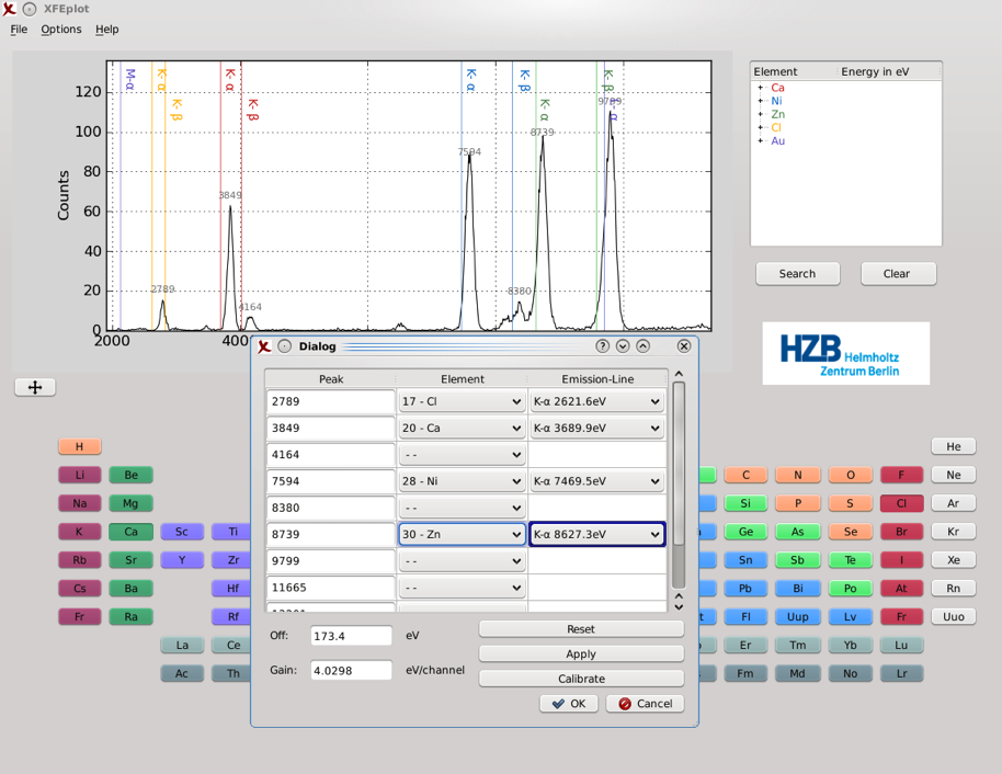
Calibration
Calibration is a tool to manually calibrate the given spectrum's energy axis. The scaling of the energy axis is determined by two parameters called offset and gain. From these two parameters, the specific energy value for each input channel of the detector is computed. The offset value sets the energy of the first channel, then for each following channel the gain value (eV/channel) is added, which leads to a linear increase over the spectrum's axes.
Computing these parameters can be done by matching peaks of known elements with the energy of their respective emission line. Via linear regression new offset and gain parameters are found which minimize the variance between each peak and emission line. It is recommended to use peaks of elements on the far left and right of the spectrum if possible, as well as multiple peaks to get the best result and least deviation.
As an example we used a test sample containing CaCl2,NiCl2 , ZnCl2 and KAuCl4 in an aqueous solution supplemented with 49% glycerol. The deviation between the peaks and the expected position is significant and one can easily see that the energy axis is badly calibrated.
After matching the peaks with their emission line, new parameters are computed and once applied the spectrum updates its energy axis.
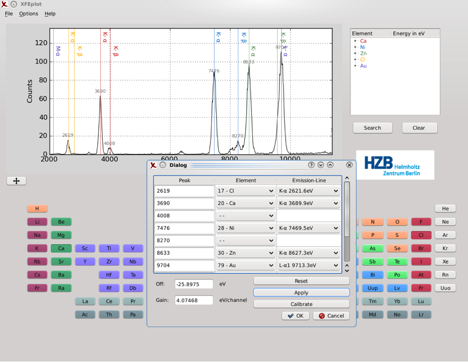
Offset and gain parameters can also be inserted manually and applied. The modified spectrum can be saved as a .dat file for later use.